Tag: python

Cramer’s Rule is a powerful method for solving systems of linear equations using determinants. It is particularly effective for small systems where calculating determinants manually is feasible. In this post, we will explain the method step-by-step and provide examples to help you master the technique.

---

What is Cramer’s Rule?

Cramer’s Rule is applicable to systems of linear equations where the number of equations matches the number of variables. The system:

   

can be expressed in matrix form as:

   

where is the coefficient matrix, is the vector of variables, and is the constants vector.

To solve for using Cramer’s Rule:

1. Compute the determinant of the coefficient matrix, .
2. Replace the -th column of with to create a new matrix .
3. Solve for each variable using the formula:

   

provided .

---

Steps to Solve Using Cramer’s Rule

1. Write the coefficient matrix and constants vector .
2. Compute .
3. For each variable :

• Replace the -th column of with\ ( \vec{b} \) to form .
• Compute .
• Solve for using .

---

Example 1: Solving a 2×2 System

Consider the system:

   

Step 1: Write the Coefficient Matrix and Constants Vector

   

Step 2: Compute

   

   

Step 3: Solve for Each Variable

• Replace the 1st column of with to get :

   

Compute :

   

   

Solve for :

   

• Replace the 2nd column of with to get :

   

Compute :

   

   

Solve for :

   

Solution:

   

Below, you can see the lines defined by this system of equations and their intersection point, which represents the solution to the system.

---

Example 2: Solving a 3×3 System

Solve the system:

   

Step 1: Write the coefficient matrix and constants vector :

   

Step 2: Compute :

   

   

Step 3: Solve for , , and :

Solve for :

Replace the first column of with :

   

   

   

   

Solve for :

Replace the second column of with :

   

   

   

   

Solve for :

Replace the third column of with :

   

   

   

   

Solution:

   

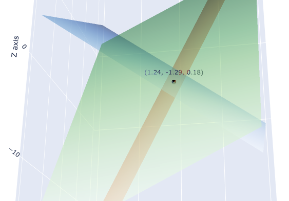
Below is an interactive plot displaying three planes defined by the system of equations, along with their intersection point, which represents the solution to the system. You can change the viewpoint by dragging the plot to explore the relationship between the planes and their intersection more effectively. Enjoy visualizing the solution!

---

Example 3: Special Case – No Solution

Solve the system:

   

Step 1: Write the coefficient matrix and constants vector :

   

Step 2: Compute :

   

   

Since , the system is inconsistent and has no solution.

Below, you can see a plot of three planes defined by this system of equations. You can change the viewpoint by dragging the plot for a better perspective. As you observe, these three planes do not intersect at any point, indicating that there is no solution for this system of equations.

---

Example 4: Special Case – Infinitely Many Solutions

Solve the system:

   

Step 1: Write the coefficient matrix and constants vector :

   

Step 2: Compute :

   

   

Since , we check consistency.

The second equation is a multiple of the first, indicating a dependency between them. As a result, the system has infinitely many solutions. Essentially, instead of three distinct equations, we only have two, which means there are two planes that intersect along a line, resulting in infinitely many solutions.Below, you can see a plot of three planes defined by this system of equations. You can change the viewpoint by dragging the plot for a better perspective. To observe the relationship between the planes, you can toggle their visibility by clicking on their names in the legend. You’ll notice that the first and second planes overlap completely. The infinitely many solutions for this system of equations can be expressed as the line 

---

Python Code

Here is the Python code to define and solve the examples above . It includes calculations for determinants and solutions for each case.

import numpy as np

# Function to compute determinant of a matrix
def determinant(matrix):
    return round(np.linalg.det(matrix), 2)

# Function to solve a system using Cramer's Rule
def cramers_rule(A, b):
    det_A = determinant(A)
    if det_A == 0:
        print("Det(A) = 0, system may have no solution or infinitely many solutions.")
        return None

    solutions = []
    n = len(b)
    for i in range(n):
        Ai = np.copy(A)
        Ai[:, i] = b
        det_Ai = determinant(Ai)
        solutions.append(det_Ai / det_A)
    return solutions

# Example 1: Solving a 2x2 System
A1 = np.array([[1, 2],
               [3, -1]])
b1 = np.array([5, 4])

print("Example 1: Solving a 2x2 System")
solutions_1 = cramers_rule(A1, b1)
if solutions_1:
    print(f"Solutions: x1 = {solutions_1[0]}, x2 = {solutions_1[1]}")

# Example 2: Solving a 3x3 System
A2 = np.array([[2, 1, -1],
               [3, -2, 4],
               [1, 3, -2]])
b2 = np.array([1, 7, -3])

print("\nExample 2: Solving a 3x3 System")
solutions_2 = cramers_rule(A2, b2)
if solutions_2:
    print(f"Solutions: x1 = {solutions_2[0]}, x2 = {solutions_2[1]}, x3 = {solutions_2[2]}")

# Example 3: No Solution
A3 = np.array([[1, 1, 1],
               [2, 2, 2],
               [1, -1, 1]])
b3 = np.array([2, 5, 1])

print("\nExample 3: No Solution")
det_A3 = determinant(A3)
if det_A3 == 0:
    print("Det(A) = 0. The system has no solution (inconsistent).")

# Example 4: Infinitely Many Solutions
A4 = np.array([[1, 1, 1],
               [2, 2, 2],
               [1, -1, 1]])
b4 = np.array([3, 6, 1])

print("\nExample 4: Infinitely Many Solutions")
det_A4 = determinant(A4)
if det_A4 == 0:
    print("Det(A) = 0. The system has infinitely many solutions (dependent equations).")