Let’s analyze the stability of a first-order system with a proportional controller using Bode Plot method. The process has a time constant of 10 seconds, and the proportional controller gain is  .
.
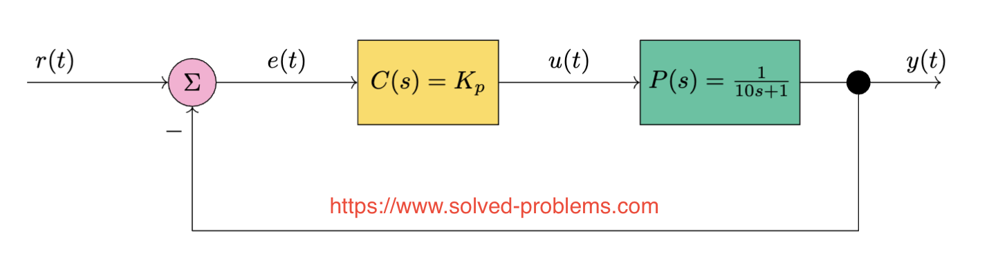
The transfer function of the process under control is:
![\[ P(s) = \frac{1}{10s + 1} \]](https://www.solved-problems.com/wp-content/ql-cache/quicklatex.com-20cd4548b46aa28be376907e4813c883_l3.png "Rendered by QuickLaTeX.com")
The transfer function of the open-loop system is:
![\[ G(s) = C(s) \cdot P(s) = \frac{K_p}{10s + 1} \]](https://www.solved-problems.com/wp-content/ql-cache/quicklatex.com-fba8f02af46ffa9e9a9b9b9d5057cc6e_l3.png "Rendered by QuickLaTeX.com")
The closed-loop transfer function is:
![\[T(s) = \frac{G(s)}{1 + G(s)} = \frac{\frac{K_p}{10s + 1}}{1 + \frac{K_p}{10s + 1}} = \frac{K_p}{10s + 1 + K_p}\]](https://www.solved-problems.com/wp-content/ql-cache/quicklatex.com-360bd60c27547fb2f6e2db68cb375dc0_l3.png "Rendered by QuickLaTeX.com")
Bode Plot and Stability Analysis for  and
and 
The Bode plot is a powerful tool used to analyze the frequency response of a control system. Even though it is drawn based on the open-loop transfer function,  (where is the controller and is the process), it provides valuable insights into the stability of the closed-loop system.
The Role of the Open-Loop Transfer Function in Closed-Loop Stability
For a system with unit feedback, the closed-loop transfer function is:
![\[ T(s) = \frac{G(s)}{1 + G(s)} = \frac{C(s)P(s)}{1 + C(s)P(s)} \]](https://www.solved-problems.com/wp-content/ql-cache/quicklatex.com-2af6d9fc6217d975cf431b99c4100a6b_l3.png "Rendered by QuickLaTeX.com")
The closed-loop system’s stability is determined by the characteristic equation:
![\[ 1 + G(s) = 1 + C(s)P(s) = 0 \]](https://www.solved-problems.com/wp-content/ql-cache/quicklatex.com-83750bcdf37574429e08625ac4ee2ad8_l3.png "Rendered by QuickLaTeX.com")
The roots of this equation (poles of the closed-loop system) dictate stability. By analyzing , we can predict whether the closed-loop poles lie in the left-half  -plane (stable) or the right-half -plane (unstable).
Key Concepts for Stability Analysis Using the Bode Plot
- Open-Loop Gain (
 ):
):
- The magnitude of
 tells how much the system amplifies signals at different frequencies.
- The magnitude of
- Phase Shift:
- The phase of shows how much delay is introduced at each frequency.
- The phase of
- Stability Margins:
- Gain Margin (GM): Indicates how much the gain of can increase before the closed-loop system becomes unstable.
- Phase Margin (PM): Indicates how much additional phase lag can be tolerated before instability occurs.
- Gain Margin (GM): Indicates how much the gain of
Steps for Stability Analysis Using the Bode Plot
- Construct the Bode Plot:
- Plot the magnitude (
 ) and phase (
 ) of across a range of frequencies (
 ).
).
- Plot the magnitude (
- Identify Critical Frequencies:
- Gain Crossover Frequency (
 ): The frequency where
  (or
(or  ).
). - Phase Crossover Frequency (
 ): The frequency where
  for
for  , or
, or  for
for  .
.
- Gain Crossover Frequency (
- Determine Stability Margins:
- Phase Margin (PM): At , measure the difference between the phase and the critical phase (
 for , for ). A positive PM indicates stability.
 - Gain Margin (GM): At , calculate the gain increase (in dB) required to make . A positive GM indicates stability.
- Phase Margin (PM): At
Why Are There Different Critical Phases for Positive and Negative Gains?
Stability analysis using the Bode plot is based on the Nyquist Stability Theorem, which states that the stability of a closed-loop system depends on the encirclement of the critical point  in the Nyquist plot.
- For : The critical phase is . The Nyquist plot must avoid encircling to ensure stability.
- For : The critical phase becomes . This accounts for the additional phase shift introduced by the negative gain.
Explanation of Critical Phase Thresholds
When :
- The phase plot starts at
 and decreases with increasing frequency.
 - Instability occurs if the total phase shift reaches , at which point the Nyquist plot risks encircling .
When :
- The negative gain introduces an additional phase shift.
- As a result, the phase plot starts at at low frequencies and decreases further.
- Instability now occurs if the total phase shift reaches , which includes the initial from the negative gain.
Thus, for , the critical phase threshold shifts from to to account for the added phase shift. This ensures consistency with the Nyquist criterion, which examines encirclement of the  point in the complex plane.
Visualizing with Nyquist Plots
Consider the Nyquist plots for  ,
,  , and
, and  :
:
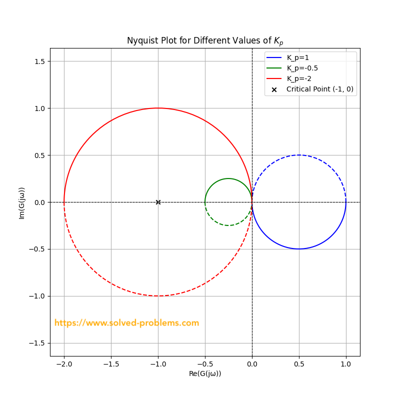
- For : The plot starts at and avoids encircling , ensuring stability.
- For : The plot starts at . Stability is maintained as it does not encircle by reaching .
- For : The plot starts at and crosses , leading to instability due to encirclement of .
This shift in the critical phase aligns with the Nyquist stability criterion and reflects the impact of the sign of on the system’s stability.
Stability Conditions for the Closed-Loop System
- The closed-loop system is stable if:
- Gain Margin

- Phase Margin

- Gain Margin
- The system is marginally stable or integrator-driven unstable if:
- Gain Margin

- Phase Margin

- Gain Margin
- The system is unstable if:
- Gain Margin
 or Phase Margin
- Gain Margin
Why the Bode Plot of  Predicts Stability of the Closed-Loop System
Although the Bode plot is based on the open-loop transfer function , it predicts closed-loop stability because the characteristic equation  involves . When has a magnitude of and a phase of , the system is on the verge of instability because it satisfies
  .
.
By ensuring sufficient gain and phase margins in the Bode plot of , you can guarantee the closed-loop poles remain in the left-half -plane.
Bode Plot for the System
For the transfer function  , the Bode plot can be derived as follows:
- Magnitude Plot:
- The magnitude of
 is:
is: ![\[ |P(j\omega)| = \frac{1}{\sqrt{(10\omega)^2 + 1}} \]](https://www.solved-problems.com/wp-content/ql-cache/quicklatex.com-29fb517985309dc5fcd756164a4227c9_l3.png "Rendered by QuickLaTeX.com")
- In decibels (dB):
![\[ 20 \log_{10} |P(j\omega)| = -20 \log_{10} \sqrt{(10\omega)^2 + 1} \]](https://www.solved-problems.com/wp-content/ql-cache/quicklatex.com-ff9a7f62be9b32890022f5324f1cd81e_l3.png "Rendered by QuickLaTeX.com")
- The magnitude of
- Phase Plot:
- The phase of is:
![\[ \angle P(j\omega) = -\tan^{-1}(10\omega) \]](https://www.solved-problems.com/wp-content/ql-cache/quicklatex.com-a40fbee3108691e1398470038dcae382_l3.png "Rendered by QuickLaTeX.com")
- The phase of
- Key Frequencies:
- At low frequencies (
 ):
):
- Magnitude:

- Phase:

- Magnitude:
- At high frequencies (
 ):
):
- Magnitude:

- Phase:

- Magnitude:
- At low frequencies (
Python Code to Generate the Bode Plot
The following Python code uses the control library to generate the Bode plot for the system:
import numpy as np
import matplotlib.pyplot as plt
from control import tf, bode

# Define the transfer function
num = [1]  # Numerator of G(s)
den = [10, 1]  # Denominator of G(s)
G = tf(num, den)

# Generate Bode plot
plt.figure()
mag, phase, omega = bode(G, dB=True, omega=np.logspace(-2, 2, 500), plot=True)

# Customize the plot
plt.suptitle("Bode Plot of the System", fontsize=14)
plt.show()
Bode plot for is depicted below:

Wait! What Happened to ?
You’re absolutely right—what happened to ? We can’t forget it! In the open-loop transfer function , we must include . Luckily, in this example, is a pure gain:  . Let’s explore how this gain impacts the Bode plot.
Magnitude Plot
The magnitude of is given by:
![\[ |G(j\omega)| = |C(j\omega)||P(j\omega)| = \frac{K_p}{\sqrt{(10\omega)^2 + 1}} \]](https://www.solved-problems.com/wp-content/ql-cache/quicklatex.com-a34728df36b0b3d61ec99a15e1aeb346_l3.png "Rendered by QuickLaTeX.com")
In decibels (dB), this becomes:
![\[ 20 \log_{10} |G(j\omega)| = 20 \log_{10} K_p - 20 \log_{10} \sqrt{(10\omega)^2 + 1} \]](https://www.solved-problems.com/wp-content/ql-cache/quicklatex.com-32c6e78b7edba5cb45993d4f26c2fe5b_l3.png "Rendered by QuickLaTeX.com")
This means the magnitude plot shifts vertically when changes. Increasing raises the plot, while decreasing lowers it.
Phase Plot
For :
The phase of is:
![\[ \angle G(j\omega) = \angle C(j\omega) - \angle P(j\omega) = 0^\circ - \tan^{-1}(10\omega) = -\tan^{-1}(10\omega) \]](https://www.solved-problems.com/wp-content/ql-cache/quicklatex.com-feb8e2d62c0573960139ecc18f74fa82_l3.png "Rendered by QuickLaTeX.com")
The phase plot for remains unchanged, as contributes no phase shift.
For :
When , the gain introduces a phase shift:
![\[ \angle G(j\omega) = \angle C(j\omega) - \angle P(j\omega) = -180^\circ - \tan^{-1}(10\omega) \]](https://www.solved-problems.com/wp-content/ql-cache/quicklatex.com-0fae7c9e42eea6958cc27022c7ae9851_l3.png "Rendered by QuickLaTeX.com")
In this case, the phase plot shifts downward by .
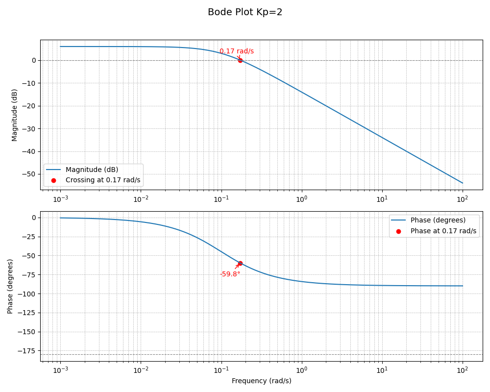
Bode Plot Analysis for
Let’s consider  . For , the magnitude plot shifts vertically with , but the phase plot remains the same.
Gain Margin:
The gain margin is  , meaning no amount of gain can make the system unstable. For instability to occur in a closed-loop system, the phase plot must cross , but this doesn’t happen here.
Phase Margin:
The phase margin measures how much additional phase lag can occur before instability. It is determined at the frequency where the magnitude crosses 0 dB.
For
At low frequencies ( ), the phase is already , and the magnitude is 0 dB. This means the phase margin is:
![\[ \text{Phase Margin} = 180^\circ -0^\circ = 180^\circ \]](https://www.solved-problems.com/wp-content/ql-cache/quicklatex.com-12e44973a8504840bc720cfe91c93d9a_l3.png "Rendered by QuickLaTeX.com")
For 
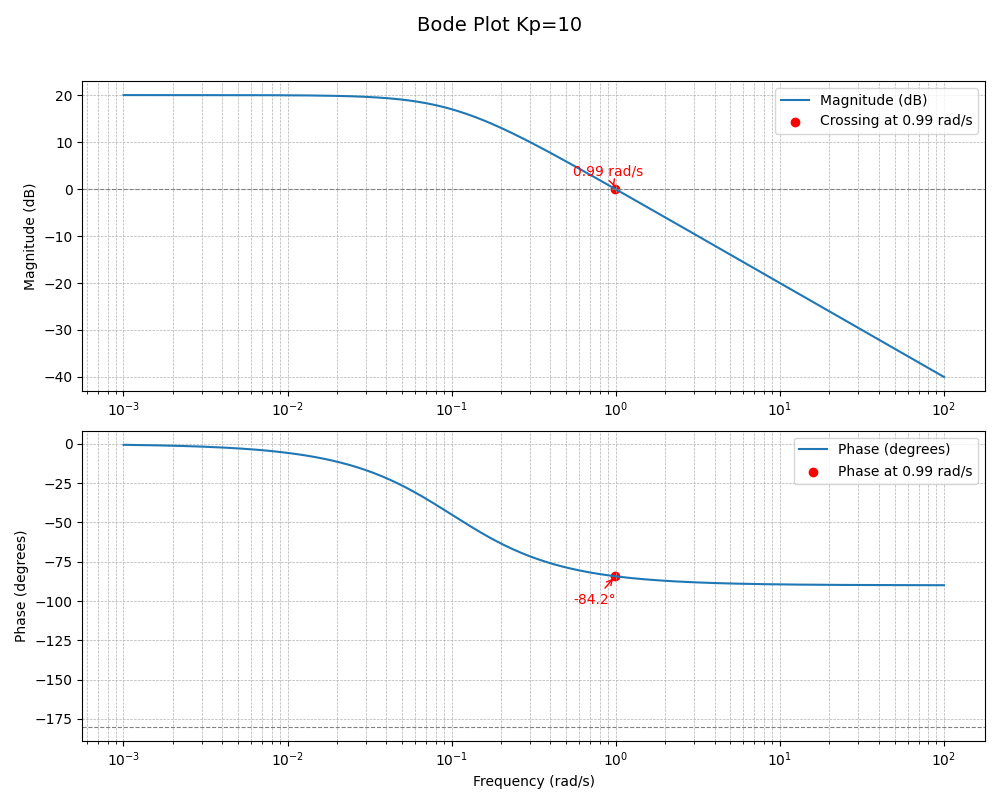
For , the magnitude crosses 0 dB at a frequency  . Solving for when :
![\[ \frac{|10|}{\sqrt{(10\omega_c)^2 + 1}} = 1 \]](https://www.solved-problems.com/wp-content/ql-cache/quicklatex.com-6e681bb6306113686e5cdb32f2032855_l3.png "Rendered by QuickLaTeX.com")
![\[ \sqrt{(10\omega_c)^2 + 1} = 10 \]](https://www.solved-problems.com/wp-content/ql-cache/quicklatex.com-9ce11158b128215a9e99f3d3b989efaa_l3.png "Rendered by QuickLaTeX.com")
![\[ (10\omega_c)^2 = 100 - 1 = 99 \]](https://www.solved-problems.com/wp-content/ql-cache/quicklatex.com-027d782668d5aace2100d6dc7b392f6f_l3.png "Rendered by QuickLaTeX.com")
![\[ \omega_c = \frac{\sqrt{99}}{10}\approx0.99 \, \text{rad/s}\]](https://www.solved-problems.com/wp-content/ql-cache/quicklatex.com-f9e7f90241aea8f2946859d944b929a2_l3.png "Rendered by QuickLaTeX.com")
The magnitude crosses 0 dB at  . At this frequency, the phase is:
![\[ \angle G(j0.99) = -\tan^{-1}(10 \cdot 0.99) \approx -84.2^\circ \]](https://www.solved-problems.com/wp-content/ql-cache/quicklatex.com-0dcc56b1ed2c9d416672962fa20b6c85_l3.png "Rendered by QuickLaTeX.com")
![\[ \text{Phase Margin} = 180^\circ - 84.2^\circ = 95.8^\circ \]](https://www.solved-problems.com/wp-content/ql-cache/quicklatex.com-19306e3002bf759dd1a779aceed4083c_l3.png "Rendered by QuickLaTeX.com")
Stability Range
The closed-loop system is stable for all because the phase plot never reaches .
What Does the Phase Margin Tell Us?
The phase margin gives us an idea of the system’s robustness. For , a phase margin of  means the system can tolerate some delay before becoming unstable.
Time Delay Interpretation
Let’s add a time delay  to the loop:
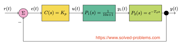
A delay introduces a phase shift proportional to frequency:
![\[ \phi = -\omega T_d \quad \text{(in radians)} \quad \text{or} \quad \phi = -\frac{180}{\pi} \cdot \omega T_d \quad \text{(in degrees)}. \]](https://www.solved-problems.com/wp-content/ql-cache/quicklatex.com-f387f80d7b4b059236c9f0bc846aeaf3_l3.png "Rendered by QuickLaTeX.com")
To reduce the phase margin by at  , the time delay is:
![\[ T_d = \frac{\phi}{-\frac{180}{\pi} \cdot \omega} \]](https://www.solved-problems.com/wp-content/ql-cache/quicklatex.com-912884a0a78bbc1781ad9d5d22b60837_l3.png "Rendered by QuickLaTeX.com")
![\[ T_d = \frac{-95.8}{-\frac{180}{\pi} \cdot 0.99} \approx 1.69 , \text{seconds}. \]](https://www.solved-problems.com/wp-content/ql-cache/quicklatex.com-3577953b2bc9da567765fc3d02ff9240_l3.png "Rendered by QuickLaTeX.com")
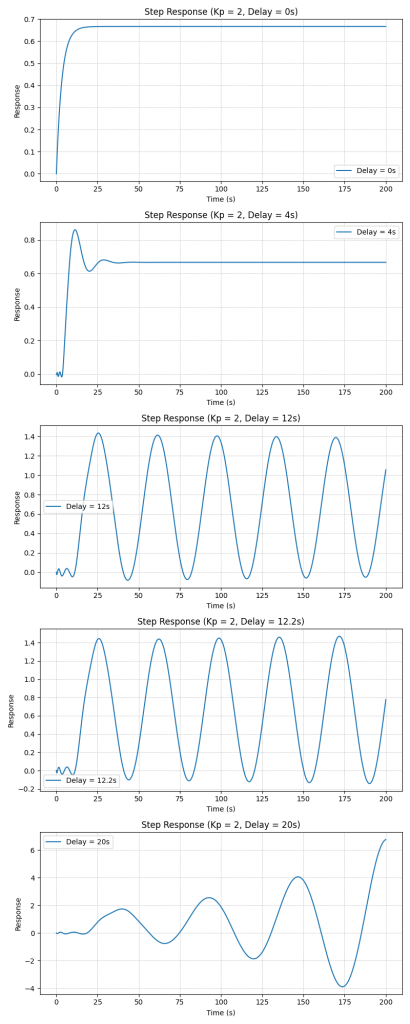
This shows that the system can tolerate a delay of approximately 1.69 seconds before losing stability when . Below, step response of the closed loop system is depicted for with various time delays.
Calculate how much delay can be added if  . You will see that the Phase margin is approximately
  that means the closed loop can tolerate 12.13 seconds of delay before becoming unstable.
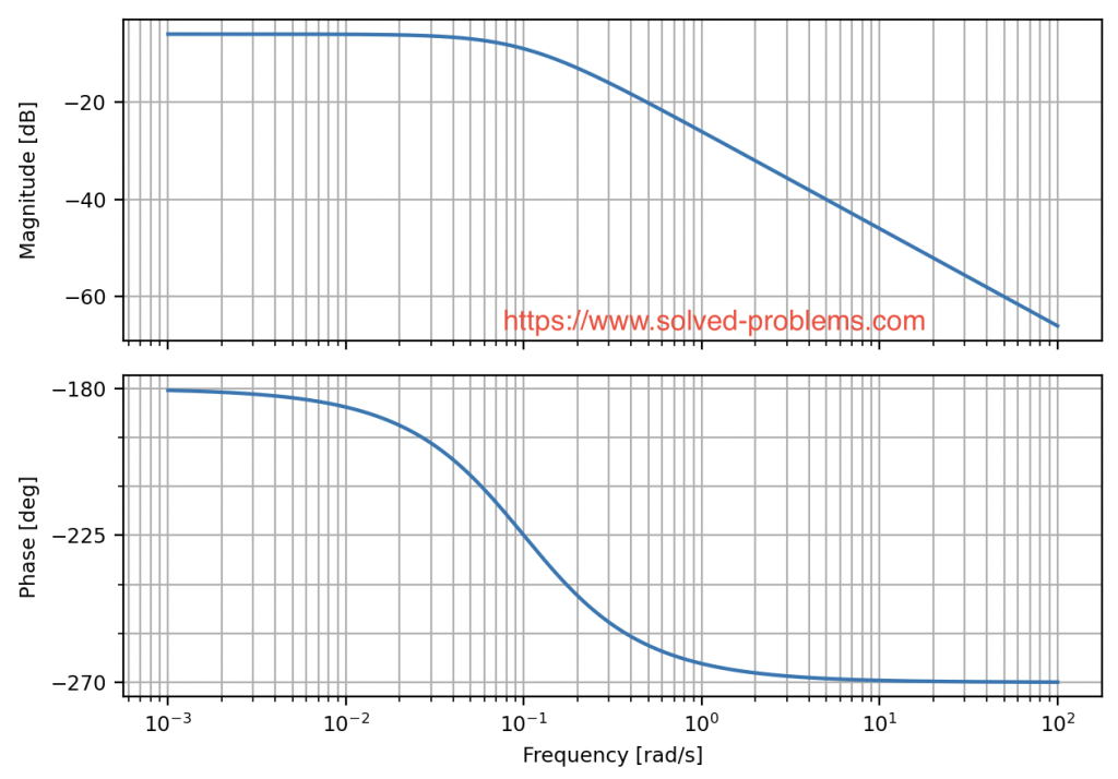
Analysis for
When , the negative gain introduces a phase shift, which affects the Bode plot as follows:
Magnitude Plot
The magnitude of remains the same because  is positive:
![\[ |G(j\omega)| = \frac{|K_p|}{\sqrt{(10\omega)^2 + 1}}. \]](https://www.solved-problems.com/wp-content/ql-cache/quicklatex.com-9c3f3d1da2701a8a414b2b7ef335e2e3_l3.png "Rendered by QuickLaTeX.com")
In decibels (dB), this is:
![\[ 20 \log_{10} |G(j\omega)| = 20 \log_{10} |K_p| - 20 \log_{10} \sqrt{(10\omega)^2 + 1}. \]](https://www.solved-problems.com/wp-content/ql-cache/quicklatex.com-f62cc09d3eed705a420d807047189cca_l3.png "Rendered by QuickLaTeX.com")
The magnitude plot shifts vertically, just as in the case, depending on .
Phase Plot
For , the phase is:
![\[ \angle G(j\omega) = \angle C(j\omega) - \angle P(j\omega) = -180^\circ - \tan^{-1}(10\omega). \]](https://www.solved-problems.com/wp-content/ql-cache/quicklatex.com-2769eb646667da51530a159c35728433_l3.png "Rendered by QuickLaTeX.com")
This means the phase plot shifts downward by , compared to the case.
Bode Plot for is depicted below.
Stability Analysis
Case 1: 
- Magnitude Plot: At low frequencies (),
 . The magnitude remains less than 1 (0 dB) because
  .
. - Phase Plot: The phase starts at and decreases further, but the closed-loop system does not cross the critical phase threshold for instability. Please refer to “Why Are There Different Critical Phases for Positive and Negative Gains?” above for more explanations.
The system is stable in this range because the Nyquist criterion is not violated.
Case 2: 
- Magnitude Plot: At low frequencies (),
 (0 dB).
 - Phase Plot: The phase starts at and decreases to
 . The system could be marginally stable or unstable because the Nyquist plot passes through the critical point. The closed loop transfer function is
. For marginal stability, poles must lie purely on the imaginary axis (e.g.,![\[T(s)=-\frac{1}{10s}\]](https://www.solved-problems.com/wp-content/ql-cache/quicklatex.com-319f82ac85950ef4e88c369a3628f19d_l3.png "Rendered by QuickLaTeX.com")
 ) and not at
  or repeated. Here, the pole at leads to integrator-driven instability, not marginal stability.
Case 3: 
- Magnitude Plot: At low frequencies (),
 (greater than 0 dB).
 - Phase Plot: The phase continues to decrease, and the Nyquist plot encircles the critical point multiple times.
The system becomes unstable for .
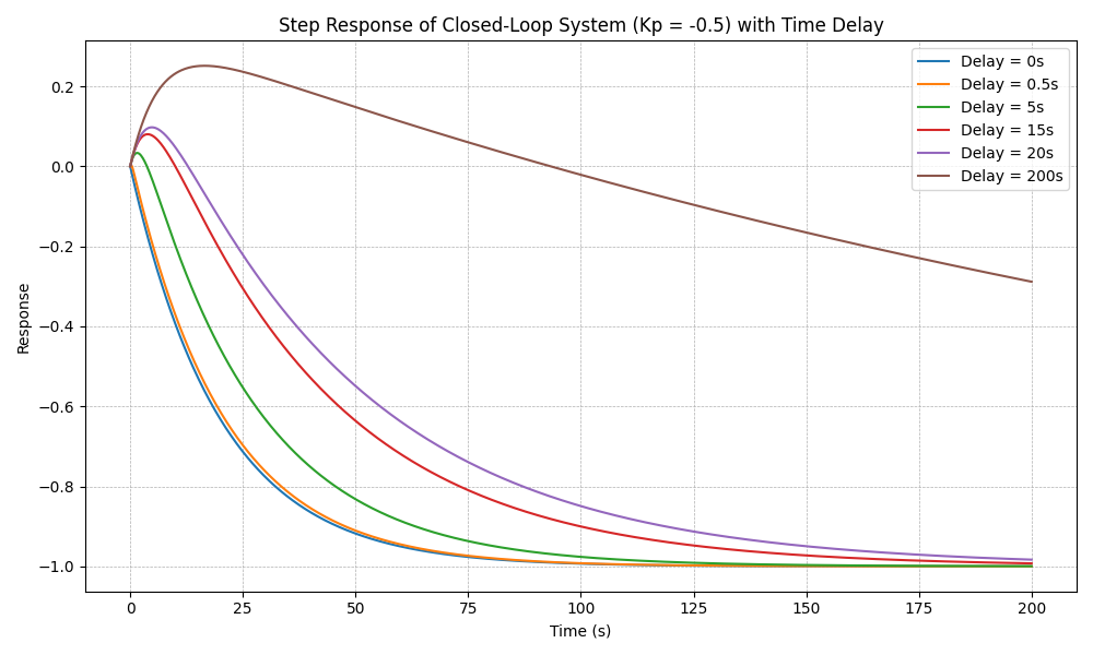
Phase Margin and Gain Margin for
Phase Margin:
For , the magnitude crosses 0 dB at a frequency . Solving for when :
![\[ \frac{|-0.5|}{\sqrt{(10\omega_c)^2 + 1}} = 1 \]](https://www.solved-problems.com/wp-content/ql-cache/quicklatex.com-faa928d2f0027ef6a50df07c54da2103_l3.png "Rendered by QuickLaTeX.com")
![\[ \sqrt{(10\omega_c)^2 + 1} = 0.5 \]](https://www.solved-problems.com/wp-content/ql-cache/quicklatex.com-f5e6b08e49f24c7e229fd0975c6155fd_l3.png "Rendered by QuickLaTeX.com")
![\[ (10\omega_c)^2 = 0.25 - 1 = -0.75 \]](https://www.solved-problems.com/wp-content/ql-cache/quicklatex.com-55f99870668257a9409f0b946c234fad_l3.png "Rendered by QuickLaTeX.com")
Since this is not physically possible, the magnitude never crosses 0 dB, and the system remains stable.
Gain Margin:
To find the gain margin, we note that the magnitude does not cross 0 dB, so the gain margin is effectively infinite.
Time Delay for Instability:
For , the phase at low frequencies is . Adding a time delay introduces a frequency-dependent phase shift:
![\[ \phi = -\omega T_d. \]](https://www.solved-problems.com/wp-content/ql-cache/quicklatex.com-d5ed0abf9b9f542323bad9681b5a3d6a_l3.png "Rendered by QuickLaTeX.com")
For instability, the phase shift must cause the total phase to reach . This means the time delay must satisfy:
![\[ -180^\circ - \omega T_d = -360^\circ. \]](https://www.solved-problems.com/wp-content/ql-cache/quicklatex.com-e3ec4de26fb318f531ae1837db65958c_l3.png "Rendered by QuickLaTeX.com")
At low frequencies ():
![\[ T_d = \frac{180^\circ}{\omega}. \]](https://www.solved-problems.com/wp-content/ql-cache/quicklatex.com-86aebaf45cee3d52a53d4b123868c747_l3.png "Rendered by QuickLaTeX.com")
Since the system remains stable at , no realistic finite time delay can destabilize it under normal conditions.
Summary
- For : The system is stable.
- For : The system is Integrator-driven instability.
- For : The system is unstable.
- For , the magnitude plot never crosses 0 dB, the phase plot shifts down by , and the system is stable with infinite gain margin and significant tolerance to time delays.
Integrator-driven instability
Integrator-driven instability occurs when a feedback control system contains an integrator in its dynamics, and the system is improperly designed, leading to unbounded growth in its response. This instability arises because the integrator accumulates input over time, and without proper control or stabilization, this accumulation can grow indefinitely.
Conclusion
The Bode plot provides a clear visualization of how the system’s frequency response changes with . The magnitude plot shifts upward as becomes more negative, while the phase plot remains unchanged. The system is stable for  , as the gain margin and phase margin are positive in this range. Beyond this range (
 ), the system becomes unstable.
The stability of the system depends on the proportional gain ():
- Stable for : the gain margin and phase margin are positive in this range.
- Integrator-driven instability for : the system is unstable.
- Unstable for
Real-World Implications of Stability
In practical applications, stability is not just a binary concept (stable or unstable). Engineers need to evaluate how stable a system is to ensure robust and reliable operation. This is where gain margin and phase margin play a crucial role.
Phase Margin and Its Importance
The phase margin (PM) provides a measure of how much additional phase delay the system can tolerate before becoming unstable. This is especially important in real-world scenarios where time delays are common.Time delay can occur due to various factors:
- Faulty sensors or actuators that respond slower than expected.
- Jammed control networks in automated systems that delay communication between components.
- Physical transport delays in processes such as chemical mixing or thermal conduction.
- External disturbances in the environment, such as varying load conditions.
When a stable system is subjected to time delays, the phase lag increases. If the phase lag reaches the critical threshold (e.g., ), the system can become unstable. The larger the phase margin, the more delay the system can tolerate before instability arises.
Gain Margin and Amplification Risks
A higher proportional gain () amplifies the system’s response but also magnifies the effects of time delay.
- With a high gain, even a small time delay can result in significant overshoot or oscillation.
- If the gain exceeds a certain limit, the system becomes unstable, as the delay causes excessive phase lag.
Example to Clarify
Imagine a factory conveyor belt controlled by an automated system.
- When the conveyor belt’s motor has a low gain, it responds sluggishly but is stable, even if the network experiences delays.
- If the motor gain is too high, the conveyor belt reacts aggressively, and even a brief network delay could cause oscillations or loss of control, resulting in spilled items or damage.
Key Takeaways
- Stable Systems Can Become Unstable with Delays: Even if a system is initially stable, time delay introduces additional phase lag, reducing phase margin. A low phase margin means even small delays can destabilize the system.
- Stability is Not Binary: Knowing how stable a system is (gain and phase margins) is critical for designing robust controllers.
- High Gain Increases Risk with Delays: While high gain improves system responsiveness, it also makes the system more sensitive to delays and disturbances, increasing the likelihood of instability.
Engineers must carefully balance stability margins and gain to ensure systems perform reliably in real-world industrial environments.
Leave a Reply