When solving systems of linear equations, the elimination method is one of the most popular and systematic approaches. This method involves adding or subtracting equations to eliminate one of the variables, allowing us to solve for the other. Once one variable is found, we substitute it back into one of the original equations to find the second variable.
Steps for Solving Using the Elimination Method
Here are the general steps for solving a system of equations using the elimination method:
- Align the equations so that like terms (variables and constants) are in columns.
- Eliminate one variable by adding or subtracting the equations. If necessary, multiply one or both equations by a constant to align coefficients.
- Solve for the remaining variable.
- Substitute the solution back into one of the original equations to find the other variable.
- Verify the solution by substituting the values into both original equations.
Example 1: A Simple Elimination Scenario
Solve the following system of equations:
![\begin{aligned}[t] 2x + 3y &= 8 \\ 4x - 3y &= 10 \end{aligned}](https://www.solved-problems.com/wp-content/ql-cache/quicklatex.com-bc8ec49f0ccf7edf0594d82caa5c3273_l3.png "Rendered by QuickLaTeX.com")
Step 1: Align the equations
The equations are already aligned:

Step 2: Eliminate one variable
Notice that the coefficients of  are opposites:
  in the first equation and
  in the second equation. To eliminate , add the two equations:

Simplify:

Step 3: Solve for 
Divide both sides by  :
:

Step 4: Solve for
Substitute into one of the original equations. Let’s use the first equation:

Simplify:

Subtract from both sides:

Divide by  :
:

Step 5: Verify the solution
Substitute and into both original equations to confirm they work:
- For
 :
: 
- For
 :
: 
Thus, the solution is:
Visualization
In the plot below, you can see the two lines represented by the equations. The point of intersection, marked on the graph, represents the solution to the system of equations.
Example 2: Multiplying to Align Coefficients
Solve the following system of equations:
![\begin{aligned}[t] 2y + 3x&= 12 \\ 5x - 4y &= -2 \end{aligned}](https://www.solved-problems.com/wp-content/ql-cache/quicklatex.com-ff1b3e2343496d59c99b4d62f2d01730_l3.png "Rendered by QuickLaTeX.com")
Step 1: Align the equations
The equations are aligned below:
![\begin{aligned}[t] 3x + 2y &= 12 \\ 5x - 4y &= -2 \end{aligned}](https://www.solved-problems.com/wp-content/ql-cache/quicklatex.com-9c46fb85cf62255db4188239af25859b_l3.png "Rendered by QuickLaTeX.com")
Step 2: Eliminate one variable
We need to align the coefficients of either or . Let’s eliminate . To do this, multiply the first equation by  and the second equation by
  (so that the coefficients of are opposites):
![\begin{aligned}[t] 2(3x + 2y) &= 2(12) \\ 1(5x - 4y) &= 1(-2) \end{aligned}](https://www.solved-problems.com/wp-content/ql-cache/quicklatex.com-d083c16ef09acab55669c713eefd0d66_l3.png "Rendered by QuickLaTeX.com")
This gives us:
![\begin{aligned}[t] 6x + 4y &= 24 \\ 5x - 4y &= -2 \end{aligned}](https://www.solved-problems.com/wp-content/ql-cache/quicklatex.com-45993ca5d00c53028794435998a133b5_l3.png "Rendered by QuickLaTeX.com")
Now, add the equations to eliminate :

Simplify:
Step 3: Solve for
Divide both sides by  :
:
Step 4: Solve for
Substitute  into one of the original equations. Let’s use the first equation:

Simplify:

Subtract from both sides:

Divide by :

Step 5: Verify the solution
Substitute and  into both original equations to confirm they work:
- For
 :
: 
- For
 :
: 
Thus, the solution is:
Visualization
The plot below illustrates the two lines corresponding to the equations. The intersection point indicates the solution to the system of equations.
Example 3: Infinite Solutions
Sometimes, a system of equations can have infinite solutions (the equations represent the same line). Let’s look at an example.
Solve the following system:
![\begin{aligned}[t] 2x + 4y &= 8 \\ x + 2y &= 4 \end{aligned}](https://www.solved-problems.com/wp-content/ql-cache/quicklatex.com-59b67ad66fa8e657f7dccfce4f0e1539_l3.png "Rendered by QuickLaTeX.com")
Step 1: Align the equations
The equations are already aligned:

Step 2: Eliminate one variable
Notice that the second equation is just half of the first. Multiply the second equation by :

Subtract the second equation from the first:

Simplify:

This is a true statement, meaning the two equations represent the same line. Therefore, there are infinite solutions.
Visualization
The plot below shows the two equations as overlapping lines, indicating that every point on the line is a solution to the system.
Example 4: No Solution
Also, a system of equations can have no solution (the lines are parallel). Here is an example.
Solve the following system of equations:
![\begin{aligned}[t] 2x + 3y &= 6 \\ 6y + 4x &= 15 \end{aligned}](https://www.solved-problems.com/wp-content/ql-cache/quicklatex.com-4e3306e629ff4a45323d7da8285471b1_l3.png "Rendered by QuickLaTeX.com")
Step 1: Align the equations
The equations are aligned below:
![\begin{aligned}[t] 2x + 3y &= 6 \ 4x + 6y &= 15 \end{aligned}](https://www.solved-problems.com/wp-content/ql-cache/quicklatex.com-dcf7c2db959eec1957996d6e8b58caf5_l3.png "Rendered by QuickLaTeX.com")
Step 2: Eliminate one variable
To eliminate one variable, we need to make the coefficients of either or the same. Let’s eliminate . Multiply the first equation by so that the coefficients of : match:
![\begin{aligned}[t] 2(2x + 3y) &= 2(6) \\ 4x + 6y &= 15 \end{aligned}](https://www.solved-problems.com/wp-content/ql-cache/quicklatex.com-86dac4293ceb9fdb9a6f15d528fee907_l3.png "Rendered by QuickLaTeX.com")
This gives us:
![\begin{aligned}[t] 4x + 6y &= 12 \\ 4x + 6y &= 15 \end{aligned}](https://www.solved-problems.com/wp-content/ql-cache/quicklatex.com-129fdac23ce5b6dbfff2d6107cdd2979_l3.png "Rendered by QuickLaTeX.com")
Now subtract the first equation from the second:

Simplify:

This is a false statement, meaning the system of equations has no solution. The two lines are parallel and never intersect.
Visualization
The plot below illustrates the two parallel lines, confirming that there is no point of intersection. This graphical representation helps to visualize why the system has no solution.
Example 5: Solving a 3×3 System of Equations
Solve the following system of equations:
![\[\begin{cases}x + 2y + z &= 8 \\2x + y - z &= 3 \\3x - y + 2z &= 7\end{cases}\]](https://www.solved-problems.com/wp-content/ql-cache/quicklatex.com-670cf71cf0b8a9a9ed4d488ebd449ac2_l3.png "Rendered by QuickLaTeX.com")
Step 1: Align the equations
The equations are already aligned:
Step 2: Eliminate one variable
We will eliminate ( z ) first. To do this, we can use the first two equations. We can add the first equation to the second equation after adjusting the coefficients of ( z ).
First, we can rewrite the second equation to align ( z ):
![\[2x + y - z = 3 \quad \text{(no change needed)}\]](https://www.solved-problems.com/wp-content/ql-cache/quicklatex.com-f4ada64d7383572e2fa9f7bace50d7dd_l3.png "Rendered by QuickLaTeX.com")
Now, we can add the first equation to the second equation:
![\[\begin{aligned}(x + 2y + z) + (2x + y - z) &= 8 + 3 \\3x + 3y &= 11\end{aligned}\]](https://www.solved-problems.com/wp-content/ql-cache/quicklatex.com-32ccc9bb94f7bfc8b42b92ea935e326d_l3.png "Rendered by QuickLaTeX.com")
Simplify:
(Eq 4) ![\[x + y = \frac{11}{3} \quad \]](https://www.solved-problems.com/wp-content/ql-cache/quicklatex.com-07485d56420abfe738067959247add55_l3.png "Rendered by QuickLaTeX.com")
Next, we will eliminate ( z ) using the first and third equations. We can rewrite the first equation to align ( z ):
![\[2x + 4y + 2z = 16 \quad \text{(multiplied by two)}\]](https://www.solved-problems.com/wp-content/ql-cache/quicklatex.com-ae7fc80b22eb15f2223866498a0b4905_l3.png "Rendered by QuickLaTeX.com")
Now, we can add the first equation to the third equation after adjusting the coefficients of ( z ):
![\[(3x - y + 2z) - (2x + 4y + 2z) &= 7 - 16\]](https://www.solved-problems.com/wp-content/ql-cache/quicklatex.com-c544c12e8c736a019a2808159f39a517_l3.png "Rendered by QuickLaTeX.com")
Simplify:
(Eq 5) ![\[x - 5y = -9 \quad \]](https://www.solved-problems.com/wp-content/ql-cache/quicklatex.com-32526e46830b33ff59e1636a964ac2db_l3.png "Rendered by QuickLaTeX.com")
Step 3: Solve for one variable
Now we have two new equations (Equation 4 and Equation 5):
 (Equation 4)
 (Equation 5)
We can solve Equation 4 for :
![\[x = \frac{11}{3} - y\]](https://www.solved-problems.com/wp-content/ql-cache/quicklatex.com-7c0b983e4009bb5cde4b821160389fb0_l3.png "Rendered by QuickLaTeX.com")
Substituting into Equation 5:
![\[\left(\frac{11}{3} - y\right) - 5y = -9\]](https://www.solved-problems.com/wp-content/ql-cache/quicklatex.com-6468bdfbe7e660dbbd78a4bf7a9ec597_l3.png "Rendered by QuickLaTeX.com")
Simplify:
![\[\frac{11}{3} - y - 5y = -9\]](https://www.solved-problems.com/wp-content/ql-cache/quicklatex.com-704b2ac8807647c034f120b9c7b14067_l3.png "Rendered by QuickLaTeX.com")
Combine like terms:
![\[\frac{11}{3} - 6y = -9\]](https://www.solved-problems.com/wp-content/ql-cache/quicklatex.com-8b925930a2d3c68f6fabf8bac68644d9_l3.png "Rendered by QuickLaTeX.com")
Multiply through by 3 to eliminate the fraction:
![\[11 - 18y = -27\]](https://www.solved-problems.com/wp-content/ql-cache/quicklatex.com-a06d2635b6425aeb289a8d16d4fe1114_l3.png "Rendered by QuickLaTeX.com")
Subtract 11 from both sides:
![\[-18y = -38\]](https://www.solved-problems.com/wp-content/ql-cache/quicklatex.com-1d8a708e90d8e134c2f994dfe5c887bc_l3.png "Rendered by QuickLaTeX.com")
Divide by -18:
![\[y = \frac{19}{9}\]](https://www.solved-problems.com/wp-content/ql-cache/quicklatex.com-4215264acf4570cb4380ecc940eca2d7_l3.png "Rendered by QuickLaTeX.com")
Step 4: Solve for and 
Substituting  back into Equation 4:
![\[x + \frac{19}{9} = \frac{11}{3}\]](https://www.solved-problems.com/wp-content/ql-cache/quicklatex.com-30c33398b783dd3cb4019a995f425427_l3.png "Rendered by QuickLaTeX.com")
Subtract  from both sides:
![\[x = \frac{11}{3} - \frac{19}{9} = \frac{33-19}{9} = \frac{14}{9}\]](https://www.solved-problems.com/wp-content/ql-cache/quicklatex.com-2fdc7e7839cea24efce5f81b058b6cb5_l3.png "Rendered by QuickLaTeX.com")
Now, substitute  and
and  back into the first original equation to find :
![\[ \frac{14}{9} + 2\left( \frac{19}{9}\right) + z = 8\]](https://www.solved-problems.com/wp-content/ql-cache/quicklatex.com-75bbbd546c68327df4919bbd86a70680_l3.png "Rendered by QuickLaTeX.com")
Simplify:
![\[ \frac{14}{9} + \frac{38}{9} + z = 8\]](https://www.solved-problems.com/wp-content/ql-cache/quicklatex.com-912a5615f48d442bfbf33c19b026bd79_l3.png "Rendered by QuickLaTeX.com")
Combine the fractions:
![\[\frac{52}{9} + z = 8\]](https://www.solved-problems.com/wp-content/ql-cache/quicklatex.com-67ffc3656739a1925b33e36a10a5e7cc_l3.png "Rendered by QuickLaTeX.com")
Subtract  from both sides:
![\[z = 8 - \frac{52}{9} = \frac{72}{9} - \frac{52}{9} = \frac{20}{9}\]](https://www.solved-problems.com/wp-content/ql-cache/quicklatex.com-f2cbce1d38d5aa8ee084785382abbd44_l3.png "Rendered by QuickLaTeX.com")
Step 5: Verify the solution
Substitute , , and  into all original equations to confirm they work:
- For
 :
:
![\[\begin{aligned}&\frac{14}{9} + 2\left(\frac{19}{9} \right) + \frac{20}{9} \\&= \frac{14}{9} + \frac{38}{9} + \frac{20}{9} \\&= \frac{14+38+20}{9} \\&= 8 \quad \text{\checkmark}\end{aligned}\]](https://www.solved-problems.com/wp-content/ql-cache/quicklatex.com-f65b8937d5e92add30b938d93ee1678f_l3.png "Rendered by QuickLaTeX.com")
- For
 :
:
![\[\begin{aligned}&2(\frac{14}{9}) + \frac{19}{9} - \frac{20}{9} \\&= \frac{28}{9} + \frac{19}{9} - \frac{20}{9} \\&= - \frac{28+19-20}{9} \\&= 3 \quad \text{\checkmark}\end{aligned}\]](https://www.solved-problems.com/wp-content/ql-cache/quicklatex.com-384c4cff6d31635011aba128086f43bc_l3.png "Rendered by QuickLaTeX.com")
- For
 :
:
![\[\begin{aligned}&3(\frac{14}{9}) - \frac{19}{9} + 2\left(\frac{20}{9} \right) \\&= \frac{42}{9} - \frac{19}{9} + \frac{40}{9} \\&= \frac{42-19+40}{3} \\&= 7 \quad \text{\checkmark}\end{aligned}\]](https://www.solved-problems.com/wp-content/ql-cache/quicklatex.com-6d693017f60eef2ad778aa9649d58866_l3.png "Rendered by QuickLaTeX.com")
Thus, the solution is: 
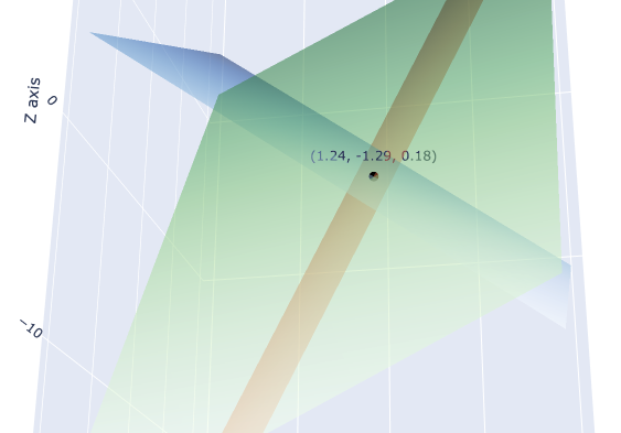
Visualization
The plot below illustrates the three planes represented by the equations. The point of intersection, marked on the graph, represents the unique solution to the system of equations.
Key Takeaways
- The elimination method is a powerful way to solve systems of equations by eliminating one variable at a time.
- Always align your equations properly and, if necessary, multiply through by constants to align coefficients.
- Verify your solution by substituting the values into both original equations.
- Keep an eye out for special cases like infinite solutions or no solution.
 .
.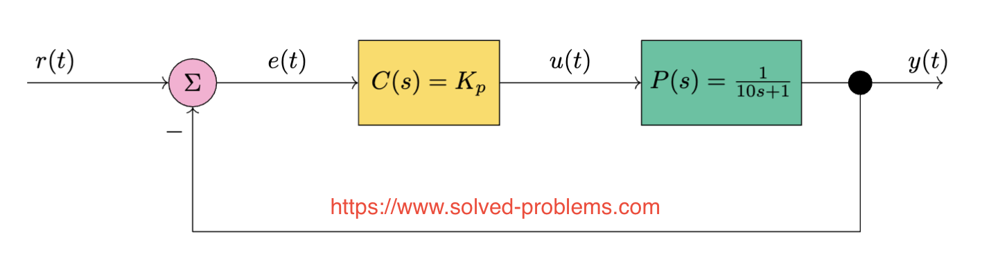
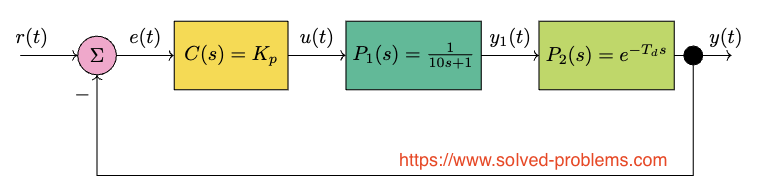
![\[ P(s) = \frac{1}{10s + 1} \]](https://www.solved-problems.com/wp-content/ql-cache/quicklatex.com-20cd4548b46aa28be376907e4813c883_l3.png "Rendered by QuickLaTeX.com")


 – resistor.

 and
and 
 and
and  are connected to the reference node through voltage sources. Therefore,
  . The same argument applies to
  .
. . We should find this value in terms of the node voltages.
  – resistor. The voltage across the resistor is
  . We prefer to define
  as
as  to comply with passive sign convention. By defining
  . Therefore,
  .
. 
 and
and  :
:


 ,
,
 :
:


 current source:
 .
. absorbing power
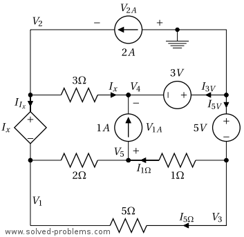
 current source:
 should be defined with polarity as indicated above. We have
  . Hence,
 supplying power.
 voltage source:
 should be defined such that it enters from the positive terminal of the source in order to use the voltage of the source in power calculation. Another option is to use

 supplying power.
 voltage source:
 should be defined as shown above to comply with the passive sign convention. We apply KCL to the reference node to find

 supplying power.
 with the direction illustrated above.
  .
.
 absorbing power.


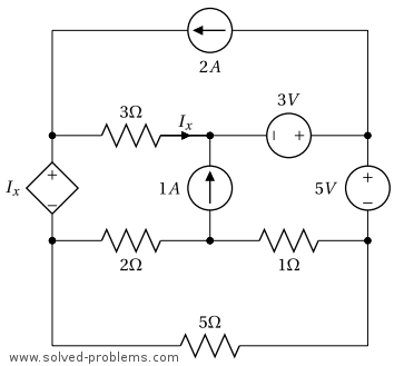
 is connected to the reference node through a voltage source. Therefore, it is equal to the voltage of the voltage source:
  .
. and
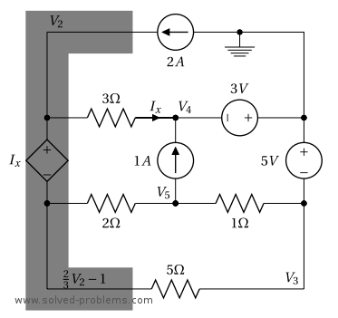
and  are connected by a voltage source. Therefore, they form a super-node. The negative terminal of the voltage source is connected to
 ![\[V_2=V_3+2.\]](https://www.solved-problems.com/wp-content/ql-cache/quicklatex.com-34cfc21f3559b4672d9081193ac694eb_l3.png "Rendered by QuickLaTeX.com")
 (the reference is always assumed to be the negative terminal of node voltages), passes through the voltage source by
  and returns back to the reference node from
![\[-V_3-2V+V_2=0 \to V_2=V_3+2.\]](https://www.solved-problems.com/wp-content/ql-cache/quicklatex.com-649ee7a294050e7fff2337ee907b9ff1_l3.png "Rendered by QuickLaTeX.com")
![\[\frac{V_3}{1\Omega}+\frac{V_3-V_4}{5\Omega}+\frac{V_2-V_1}{2\Omega}+\frac{V_2-V_5}{3\Omega}=0\]](https://www.solved-problems.com/wp-content/ql-cache/quicklatex.com-f1e91d3309112c978773d54024fb90cd_l3.png "Rendered by QuickLaTeX.com")
![\[\to {V_3}+\frac{V_3}{5}-\frac{V_4}{5}+\frac{V_3+2-10}{2}+\frac{V_3+2-V_5}{3}=0\]](https://www.solved-problems.com/wp-content/ql-cache/quicklatex.com-5566abcbbd54661d3cf5427f8967b0a9_l3.png "Rendered by QuickLaTeX.com")
![\[\to {V_3}+\frac{V_3}{5}-\frac{V_4}{5}+\frac{V_3}{2}-4+\frac{V_3}{3}+\frac{2}{3}-\frac{V_5}{3}=0\]](https://www.solved-problems.com/wp-content/ql-cache/quicklatex.com-845d693cfddc8403a4e3f4882c29e1d5_l3.png "Rendered by QuickLaTeX.com")
![\[\to \frac{61}{30}V_3-\frac{V_4}{5}-\frac{V_5}{3}=\frac{10}{3}\]](https://www.solved-problems.com/wp-content/ql-cache/quicklatex.com-2e7c80e6818ab31cfe670af42424a3c3_l3.png "Rendered by QuickLaTeX.com")
![\[\to 61 V_3-6 V_4-10 V_5=100\]](https://www.solved-problems.com/wp-content/ql-cache/quicklatex.com-89072ddb695ffe2deb098c693f542b69_l3.png "Rendered by QuickLaTeX.com")
 :
:![\[\frac{V_4}{6\Omega}+\frac{V_4-V_3}{5\Omega}+10=0\]](https://www.solved-problems.com/wp-content/ql-cache/quicklatex.com-568fa5bd8e36e406bd2f86249060293d_l3.png "Rendered by QuickLaTeX.com")
![\[\to 5 V_4+6 V_4-6V_3+300=0\]](https://www.solved-problems.com/wp-content/ql-cache/quicklatex.com-0d7b5dfb55702ea7f0a8eb47e8cc88f1_l3.png "Rendered by QuickLaTeX.com")
![\[\to -6V_3+11 V_4=-300\]](https://www.solved-problems.com/wp-content/ql-cache/quicklatex.com-53f7f294b731212be42c22ddadfdc3c1_l3.png "Rendered by QuickLaTeX.com")
 :
:![\[\frac{V_5}{4\Omega}+\frac{V_5-V_2}{3\Omega}-10=0\]](https://www.solved-problems.com/wp-content/ql-cache/quicklatex.com-774066816a5c0acef1d4335a1c28ca84_l3.png "Rendered by QuickLaTeX.com")
![\[\to 3V_5+4V_5-4V_2-120=0\]](https://www.solved-problems.com/wp-content/ql-cache/quicklatex.com-9b7eacd0118f6ad1ca26dcf10e3972bf_l3.png "Rendered by QuickLaTeX.com")
![\[\to 7V_5-4 V_3-8-120=0\]](https://www.solved-problems.com/wp-content/ql-cache/quicklatex.com-29c998f696da9f88931811251d6e92e9_l3.png "Rendered by QuickLaTeX.com")
![\[\to -4 V_3+7V_5=128\]](https://www.solved-problems.com/wp-content/ql-cache/quicklatex.com-31d31c06b3fa61fac3f2126275f43d48_l3.png "Rendered by QuickLaTeX.com")
![\[\left\{ \begin{array}{l} 61 V_3-6 V_4-10 V_5=100 \\ -6V_3+11 V_4=-300 \\ -4 V_3+7V_5=128 \end{array} \right.\]](https://www.solved-problems.com/wp-content/ql-cache/quicklatex.com-265860250d9eab754e916d35e60577c6_l3.png "Rendered by QuickLaTeX.com")


![Thus, [latex]V_2=V_3+2=4.292.](https://www.solved-problems.com/wp-content/ql-cache/quicklatex.com-29edb764dc83c14df778ad3f3f7f080c_l3.png "Rendered by QuickLaTeX.com")
 Source:
 resistor. Using Ohm’s Law, this current is:
![\[I_{10 \, \mathrm{V}} = \frac{V_2 - V_1}{2 \, \Omega} = -2.854 \, \mathrm{A}.\]](https://www.solved-problems.com/wp-content/ql-cache/quicklatex.com-ffe9ad653492ff77b714d326f3bea820_l3.png "Rendered by QuickLaTeX.com")
![\[P_{10 \, \mathrm{V}} = 10 \times (-2.854) = -28.54 \, \mathrm{W}.\]](https://www.solved-problems.com/wp-content/ql-cache/quicklatex.com-9694d039de3822345ac308ddb7b1dc68_l3.png "Rendered by QuickLaTeX.com")
 Source:
 and
and  resistors. Using Ohm’s Law, we calculate:
![\[I_{2 \, \mathrm{V}} = I_{5 \, \Omega} + I_{1 \, \Omega} = \frac{V_3 - V_4}{5 \, \Omega} + \frac{V_3}{1 \, \Omega}.\]](https://www.solved-problems.com/wp-content/ql-cache/quicklatex.com-9f3093d9504b0c689f1cd276c5f8e3ef_l3.png "Rendered by QuickLaTeX.com")
![\[I_{2 \, \mathrm{V}} = 5.663 + 2.292 = 7.955 \, \mathrm{A}.\]](https://www.solved-problems.com/wp-content/ql-cache/quicklatex.com-9c7e12f483d5f5647ba6e0f48c8e0314_l3.png "Rendered by QuickLaTeX.com")
![\[P_{2 \, \mathrm{V}} = 2 \times 7.955 = 15.91 \, \mathrm{W}.\]](https://www.solved-problems.com/wp-content/ql-cache/quicklatex.com-d7e2a76aeaadf66b99bd8630599a0c70_l3.png "Rendered by QuickLaTeX.com")
 Current Source:
![\[V_{10 \, \mathrm{A}} = V_4 - V_5 = -45.617 \, \mathrm{V}.\]](https://www.solved-problems.com/wp-content/ql-cache/quicklatex.com-2c4d88fa8e030f45ec0505852880de3d_l3.png "Rendered by QuickLaTeX.com")
![\[P_{10 \, \mathrm{A}} = 10 \times (-45.617) = -456.17 \, \mathrm{W}.\]](https://www.solved-problems.com/wp-content/ql-cache/quicklatex.com-e479ec9d7227df7bef098696b8bc745f_l3.png "Rendered by QuickLaTeX.com")


![\[\begin{cases}a_{11}x_1 + a_{12}x_2 + \dots + a_{1n}x_n = b_1 \\a_{21}x_1 + a_{22}x_2 + \dots + a_{2n}x_n = b_2 \\\vdots \\a_{n1}x_1 + a_{n2}x_2 + \dots + a_{nn}x_n = b_n\end{cases}\]](https://www.solved-problems.com/wp-content/ql-cache/quicklatex.com-97d043977401f9612fa18a9affc8b93d_l3.png "Rendered by QuickLaTeX.com")
![\[A \vec{x} = \vec{b},\]](https://www.solved-problems.com/wp-content/ql-cache/quicklatex.com-e88dd01f236f8f653ac3a5956be74d32_l3.png "Rendered by QuickLaTeX.com")
 is the coefficient matrix,
  is the vector of variables, and
  is the constants vector.
 using Cramer’s Rule:
 .
. -th column of
  .
.![\[x_i = \frac{\det(A_i)}{\det(A)},\]](https://www.solved-problems.com/wp-content/ql-cache/quicklatex.com-61f7e8ae81d9a78fff2cc42c7e9db2e6_l3.png "Rendered by QuickLaTeX.com")
 .
. :
: .
. .
.![\[\begin{cases}x + 2y = 5 \\3x - y = 4\end{cases}\]](https://www.solved-problems.com/wp-content/ql-cache/quicklatex.com-1d2de21cce6ab26e5b4520db96b0ab29_l3.png "Rendered by QuickLaTeX.com")
![\[A = \begin{bmatrix}1 & 2 \\3 & -1\end{bmatrix}, \quad \vec{b} = \begin{bmatrix} 5 \ 4 \end{bmatrix}.\]](https://www.solved-problems.com/wp-content/ql-cache/quicklatex.com-cc3538d77f8c05c25ddd7b8acb4f7425_l3.png "Rendered by QuickLaTeX.com")
![\[\det(A) = \begin{vmatrix}1 & 2 \\3 & -1\end{vmatrix}\]](https://www.solved-problems.com/wp-content/ql-cache/quicklatex.com-bf1cfc09f0d4d0f313cf507fe43dc2a6_l3.png "Rendered by QuickLaTeX.com")
![\[\det(A) = (1)(-1) - (2)(3) = -1 - 6 = -7.\]](https://www.solved-problems.com/wp-content/ql-cache/quicklatex.com-f6916f517ec4105b72c9dcc35cfef6bc_l3.png "Rendered by QuickLaTeX.com")
 :
:![\[A_1 = \begin{bmatrix}5 & 2 \\4 & -1\end{bmatrix}.\]](https://www.solved-problems.com/wp-content/ql-cache/quicklatex.com-6843560e8e67747a87dc1f9d84db30b9_l3.png "Rendered by QuickLaTeX.com")
 :
:![\[\det(A_1) = \begin{vmatrix}5 & 2 \\4 & -1\end{vmatrix}\]](https://www.solved-problems.com/wp-content/ql-cache/quicklatex.com-251641b2ad3a256655cf9896d359f77b_l3.png "Rendered by QuickLaTeX.com")
![\[\det(A_1) = (5)(-1) - (2)(4) = -5 - 8 = -13.\]](https://www.solved-problems.com/wp-content/ql-cache/quicklatex.com-a026fa860410e13838500a66c641d166_l3.png "Rendered by QuickLaTeX.com")
![\[x = \frac{\det(A_1)}{\det(A)} = \frac{-13}{-7} = \frac{13}{7}.\]](https://www.solved-problems.com/wp-content/ql-cache/quicklatex.com-d6b00459c7184041c4081d84d656fea0_l3.png "Rendered by QuickLaTeX.com")
 :
:![\[A_2 = \begin{bmatrix}1 & 5 \\3 & 4\end{bmatrix}.\]](https://www.solved-problems.com/wp-content/ql-cache/quicklatex.com-e4be0e03bc03b1ba6ad81f51ddc62dbe_l3.png "Rendered by QuickLaTeX.com")
 :
:![\[\det(A_2) = \begin{vmatrix}1 & 5 \\3 & 4\end{vmatrix}.\]](https://www.solved-problems.com/wp-content/ql-cache/quicklatex.com-2ad9b82e41e570abc8c1e6fd3ff0af85_l3.png "Rendered by QuickLaTeX.com")
![\[\det(A_2) = (1)(4) - (5)(3) = 4 - 15 = -11.\]](https://www.solved-problems.com/wp-content/ql-cache/quicklatex.com-79d3a5f7040633f523d47d3aa37b3e1a_l3.png "Rendered by QuickLaTeX.com")
![\[y = \frac{\det(A_2)}{\det(A)} = \frac{-11}{-7} = \frac{11}{7}.\]](https://www.solved-problems.com/wp-content/ql-cache/quicklatex.com-424cdd3bc903ffbef94a1a268e978d87_l3.png "Rendered by QuickLaTeX.com")
![\[x = \frac{13}{7}, \quad y = \frac{11}{7}.\]](https://www.solved-problems.com/wp-content/ql-cache/quicklatex.com-edbb08c81b004c899f8bc08740c7c60e_l3.png "Rendered by QuickLaTeX.com")

![\[\begin{cases}2x + y - z &= 1, \\3x - 2y + 4z &= 7, \\x + 3y - 2z &= -3.\end{cases}\]](https://www.solved-problems.com/wp-content/ql-cache/quicklatex.com-63148886e50dccba76909971a1a33e5b_l3.png "Rendered by QuickLaTeX.com")
![\[A = \begin{bmatrix}2 & 1 & -1 \\3 & -2 & 4 \\1 & 3 & -2\end{bmatrix}, \quad\vec{b} = \begin{bmatrix}1 \ 7 \ -3\end{bmatrix}.\]](https://www.solved-problems.com/wp-content/ql-cache/quicklatex.com-c4f7dc8db40136b7dc0830ab78b2476b_l3.png "Rendered by QuickLaTeX.com")
![\[\begin{split}\det(A) = &2(-2 \times -2 - 4 \times 3) \\&- 1(3 \times -2 - 4 \times 1) \\&- 1(3 \times 3 - (-2 \times 1)).\end{split}\]](https://www.solved-problems.com/wp-content/ql-cache/quicklatex.com-7e6f3493236bdaa29628c3a9d7883f6a_l3.png "Rendered by QuickLaTeX.com")
![\[\begin{split}\det(A) &= 2(4 - 12) - 1(-6 - 4) - 1(9 + 2) \\&= 2(-8) + 10 - 11 \\ &= -16 + 10 - 11 \\&= -17.\end{split}\]](https://www.solved-problems.com/wp-content/ql-cache/quicklatex.com-b06feb47bb4a8485aac5559871b62d37_l3.png "Rendered by QuickLaTeX.com")
 ,
,  , and
, and  :
:![\[A_1 = \begin{bmatrix}1 & 1 & -1 \\7 & -2 & 4 \\-3 & 3 & -2\end{bmatrix}.\]](https://www.solved-problems.com/wp-content/ql-cache/quicklatex.com-04f773ecc029ab003a869f6477812d5a_l3.png "Rendered by QuickLaTeX.com")
![\[\begin{split}\det(A_1) = &1(-2 \times -2 - 4 \times 3) \\&- 1(7 \times -2 - 4 \times -3) \\&+ (-1)(7 \times 3 - (-2 \times -3)).\end{split}\]](https://www.solved-problems.com/wp-content/ql-cache/quicklatex.com-070b1fd4066483e47650f91f14df61ad_l3.png "Rendered by QuickLaTeX.com")
![\[\begin{split}\det(A_1) &= 1(4 - 12) - 1(-14 + 12) - (21 - 6) \\&= -8 + 2 - 15 \\&= -21.\end{split}\]](https://www.solved-problems.com/wp-content/ql-cache/quicklatex.com-269adc73905ad44f54b439e556482514_l3.png "Rendered by QuickLaTeX.com")
![\[x_1 = \frac{\det(A_1)}{\det(A)} = \frac{-21}{-17} = \frac{21}{17}.\]](https://www.solved-problems.com/wp-content/ql-cache/quicklatex.com-8490a67f89471f7cb75f90c600094819_l3.png "Rendered by QuickLaTeX.com")
![\[A_2 = \begin{bmatrix}2 & 1 & -1 \\3 & 7 & 4 \\1 & -3 & -2\end{bmatrix}.\]](https://www.solved-problems.com/wp-content/ql-cache/quicklatex.com-b1ffe3eb8d53f0640d9f702ab7e92cf5_l3.png "Rendered by QuickLaTeX.com")
![\[\begin{split}\det(A_2) = &2(7 \times -2 - 4 \times -3) \\&- 1(3 \times -2 - 4 \times 1) \\&+ (-1)(3 \times -3 - 7 \times 1).\end{split}\]](https://www.solved-problems.com/wp-content/ql-cache/quicklatex.com-39bef044188e00db0b82424eb41f138c_l3.png "Rendered by QuickLaTeX.com")
![\[\begin{split}\det(A_2) &= 2(-14 +12) - 1(-6 - 4) - 1(-9 - 7) \\&= 2(-2) + 10 +16 \\&= -4 + 10 + 16 \\&= 22.\end{split}\]](https://www.solved-problems.com/wp-content/ql-cache/quicklatex.com-6a4c92976f24cbe94601f9fd0bf90a6b_l3.png "Rendered by QuickLaTeX.com")
![\[x_2 = \frac{\det(A_2)}{\det(A)} = \frac{22}{-17} = -\frac{22}{17}.\]](https://www.solved-problems.com/wp-content/ql-cache/quicklatex.com-00d48de22675a1333a90d535eb025380_l3.png "Rendered by QuickLaTeX.com")
![\[A_3 = \begin{bmatrix}2 & 1 & 1 \\3 & -2 & 7 \\1 & 3 & -3\end{bmatrix}.\]](https://www.solved-problems.com/wp-content/ql-cache/quicklatex.com-b34572107f0ba5ad288936f0a7179b39_l3.png "Rendered by QuickLaTeX.com")
![\[\begin{split}\det(A_3) = &2(-2 \times -3 - 7 \times 3) \\&- 1(3 \times -3 - 7 \times 1) \\&+ 1(3 \times 3 - (-2 \times 1)).\end{split}\]](https://www.solved-problems.com/wp-content/ql-cache/quicklatex.com-9d8ce91e2f80400e4c71a0621729527a_l3.png "Rendered by QuickLaTeX.com")
![\[\begin{split}\det(A_3) &= 2(6 - 21) - 1(-9 - 7) + 1(9 + 2) \\&= 2(-15) + 16 + 11 \\&= -30 + 16 + 11 \\&= -3.\end{split}\]](https://www.solved-problems.com/wp-content/ql-cache/quicklatex.com-a9b8410a6883b49c96e29b196b9d484c_l3.png "Rendered by QuickLaTeX.com")
![\[x_3 = \frac{\det(A_3)}{\det(A)} = \frac{-3}{-17} = \frac{3}{17}.\]](https://www.solved-problems.com/wp-content/ql-cache/quicklatex.com-db9e5df79387a13b75d823a60af7e91f_l3.png "Rendered by QuickLaTeX.com")
![\[x_1 = \frac{21}{17}, \quad x_2 = -\frac{22}{17}, \quad x_3 = \frac{3}{17}.\]](https://www.solved-problems.com/wp-content/ql-cache/quicklatex.com-0064c2c183c9bde3fd0428d621dd349a_l3.png "Rendered by QuickLaTeX.com")
![\[\begin{cases}x + y + z &= 2, \\2x + 2y + 2z &= 5, \\x - y + z &= 1.\end{cases}\]](https://www.solved-problems.com/wp-content/ql-cache/quicklatex.com-96ee6b99b6aaeff01c72b687b16ade6f_l3.png "Rendered by QuickLaTeX.com")
![\[A = \begin{bmatrix}1 & 1 & 1 \\2 & 2 & 2 \\1 & -1 & 1\end{bmatrix}, \quad\vec{b} = \begin{bmatrix}2 \ 5 \ 1\end{bmatrix}.\]](https://www.solved-problems.com/wp-content/ql-cache/quicklatex.com-8183ba0bea98211386ab5eff2bdd919d_l3.png "Rendered by QuickLaTeX.com")
![\[\begin{split}\det(A) &= 1(2 \times 1 - 2 \times -1) \\&- 1(2 \times 1 - 2 \times 1) \\&+ 1(2 \times -1 - 2 \times 1).\end{split}\]](https://www.solved-problems.com/wp-content/ql-cache/quicklatex.com-ef8f5a32175cb45334a79e21a86cce2c_l3.png "Rendered by QuickLaTeX.com")
![\[\det(A) = 1(2 + 2) - 1(2 - 2) + 1(-2 - 2) = 4 - 0 - 4 = 0.\]](https://www.solved-problems.com/wp-content/ql-cache/quicklatex.com-85df8361220f8856191860748121b7ef_l3.png "Rendered by QuickLaTeX.com")
 , the system is inconsistent and has no solution.
![\[\begin{cases}x + y + z &= 3, \\2x + 2y + 2z &= 6, \\x - y + z &= 1.\end{cases}\]](https://www.solved-problems.com/wp-content/ql-cache/quicklatex.com-89fe91bafef4e6274efc429a63f64d87_l3.png "Rendered by QuickLaTeX.com")
![\[A = \begin{bmatrix}1 & 1 & 1 \\2 & 2 & 2 \\1 & -1 & 1\end{bmatrix}, \quad\vec{b} = \begin{bmatrix}3 \ 6 \ 1\end{bmatrix}.\]](https://www.solved-problems.com/wp-content/ql-cache/quicklatex.com-d99e9cd2bc42f4893f091c69781a6dfd_l3.png "Rendered by QuickLaTeX.com")
![\[\begin{split}\det(A) =& 1(2 \times 1 - 2 \times -1) \\&- 1(2 \times 1 - 2 \times 1) \\&+ 1(2 \times -1 - 2 \times 1).\end{split}\]](https://www.solved-problems.com/wp-content/ql-cache/quicklatex.com-22ecca84025676a297dacb93c4ccb97b_l3.png "Rendered by QuickLaTeX.com")
![\[\begin{split}\det(A) &= 1(2 + 2) - 1(2 - 2) + 1(-2 - 2) \\&= 4 - 0 - 4 \\&= 0.\end{split}\]](https://www.solved-problems.com/wp-content/ql-cache/quicklatex.com-0e8f881cd5ec6f6da44b65bf383f3d3f_l3.png "Rendered by QuickLaTeX.com")


 .
.
